pde.h File Reference
Class PDE: the differential equation object. More...
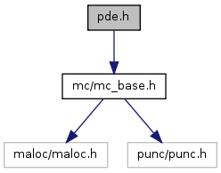
#include <mc/mc_base.h>
Include dependency graph for pde.h:
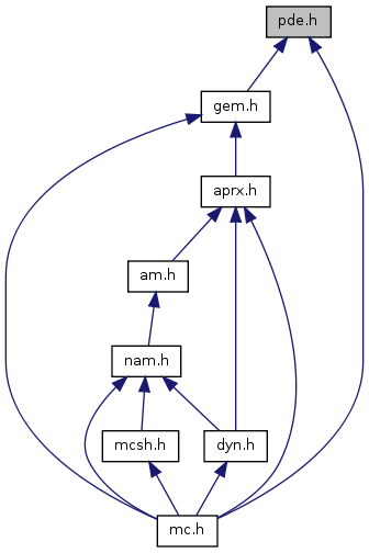
This graph shows which files directly or indirectly include this file:
Go to the source code of this file.
Classes | |
| struct | sPDE |
| Class PDE: Definition. More... | |
Typedefs | |
| typedef struct sPDE | PDE |
| Declaration of the PDE class as the PDE structure. | |
Functions | |
| void | PDE_setDim (PDE *thee, int d) |
| Set the extrinsic spatial dimension. | |
| void | PDE_setDimII (PDE *thee, int d) |
| Set the extrinsic spatial dimension. | |
| int | PDE_dim (PDE *thee) |
| Return the extrinsic spatial dimension. | |
| int | PDE_dimII (PDE *thee) |
| Return the extrinsic spatial dimension. | |
| int | PDE_vec (PDE *thee) |
| Return the PDE product space dimension. | |
| PDE * | PDE_ctor_default (void) |
| Construct a fake differential equation object in case there is not one provided. | |
| void | PDE_dtor_default (PDE **thee) |
| Destroy a fake differential equation object. | |
| int | PDE_sym (PDE *thee, int i, int j) |
| Return the bilinear form minor symmetry (i,j). | |
Detailed Description
Class PDE: the differential equation object.
- Note:
 *           The differential operator information is provided by
 *           specifying the following:
 *
 *       vec               Product dim (unknowns per spatial point)
 *       sym[MAXV][MAXV];  Symmetry/nonsymmetry of bilinear form
 *
 *       initAssemble      Once-per-assembly initialization
 *       initElement       Once-per-element initialization
 *       initFace          Once-per-face initialization
 *       initPoint         Once-per-point (e.g. quadrature pt) initialization
 *
 *       Fu                The nonlinear strong form defining the PDE
 *       Ju                The nonlinear energy (PDE is the Euler condition)
 *       Fu_v              The nonlinear weak form defining the PDE
 *       DFu_wv            The bilinear linearization weak form
 *       delta             The delta function source term (if present)
 *       u_D               The dirichlet boundary condition function
 *       u_T               Optional analytical solution function (for testing)
 *
 *       bisectEdge        The rule used to spit edges of simplices
 *       mapBoundary       The rule used to recover boundary surfaces exactly
 *       markSimplex       The rule used to mark simplices for refinement
 *       oneChart          Coordinate transformations
 *
 *       simplexBasisInit  Trial and test space bases initialization
 *       simplexBasisForm  Trial and test space bases formation
 *
 *          The following two additional parameters are determined by the
 *          input manifold, and are then set appropriately to be available
 *          to the user's PDE definition routines above:
 *
 *       dim               Manifold intrinsic dim (determined by mesh input)
 *       dimII             Manifold imbedding dim (determined by mesh input)
 *
 * Notes on the forms: Fu_v/DFu_wv
 *
 *           At the single given point x, we must evaluate the functionals
 *
 *               Fu_v   = F(u)(v)    = F (x, u(x),grad u(x), v(x),grad v(x))
 *
 *               DFu_wv = DF(u)(w,v) = DF(x, u(x),grad u(x), v(x),grad v(x),
 *                                           w(x),grad w(x))
 *
 *           The functional F(u)(v):HxH-->R is assumed to be linear in
 *           the argument v, but possibly nonlinear in the argument u.
 *
 *           The functional DF(u)(w,v):HxHxH-->R is assumed to be linear in
 *           the arguments v and w, but possibly nonlinear in the argument u.
 *
 *           Here, H is some Banach space of functions, such as the
 *           Sobolev space W^{1,p}(\Omega), 1<=p<\infty, or some product
 *           space based on these spaces.
 *
 * The forms Fu_v/DFu_wv and their use in Newton iterations:
 *
 *           The functional F(u)(v) is a weak formulation of some nonlinear
 *           partial differential equation.  This functional represents a
 *           nonlinear operator in an equation of the form:
 *
 *               (P1) Find u in H such that F(u)(v)=0 for all v in H.
 *
 *           As a function of its first argument only, the functional F(u)(v)
 *           can be viewed as a mapping from the space H into the space of
 *           linear functionals on H, or F(u)(v):H->L(H,R).  Similarly, the
 *           Frechet derivative of F(u)(v) with respect to u represents a
 *           mapping DF(u)(w,v):H->L(HxH,R), which is a mapping from H into
 *           the space of bilinear forms on H.  At a point z in H, such a
 *           bilinear form will be denoted:
 *
 *               DF(z)(u,v).
 *
 *           A Newton iteration for solving (P1) takes the form:
 *
 *               (0) Given some initial guess of u in H.
 *                   (For linear problems, we will always start with u=0.)
 *               (1) Find w in H such that DF(u)(w,v)=-F(u)(v), for all v in H.
 *               (2) Update u:  u = u + w
 *               (3) If (F(u)(v)>TOL) for some v in H, goto (1)
 *               (4) Quit
 *
 *           If this is a linear problem, in that F(u)(v) is only affine in the
 *           argument u rather than truly nonlinear, then the operator has
 *           the general form:
 *
 *               F(u)(v) = A(u,v) - (f,v),
 *
 *           where A(u,v) is bilinear.  Therefore, problem (P1) has the form:
 *
 *               (P2) Find u in H such that A(u,v)=(f,v) for all v in H.
 *
 *           The Frechet derivative of F(u)(v) with respect to u at a point z
 *           is simply the bilinear form (independent of z)
 *
 *               DF(z)(u,v) = A(u,v).
 *
 *           Now, since we will require u=0 to start a Newton iteration for a
 *           linear problem, this will produce the linear source term as
 *           required to solve the linear problem:
 *
 *               (Aw,v) = DF(0)(w,v) = -F(0)(v) = (f,v)
 *
 *           So, Step (1) in our Newton iteration will be exactly the
 *           solution of the linear problem (P2), which is the proper
 *           linearization of a linear (affine) problem.  Step (2) of the
 *           Newton iteration them forms u as u=0+w, and Step (3) then sees
 *           F(u)(v)=A(w,v)-(f,v)=0, which leads to completion in Step (4).
 *
 * Sub-form implementation of Fu_v/DFu_wv and computational details:
 *
 *           For the sake of efficiency, these forms may be implemented in
 *           terms of sub-forms on orthogonal spaces.  For systems of partial
 *           differential equations, the functions u,v,w above have the form:
 *
 *               u=(u_1, u_2, ... , u_m),
 *
 *           so that u then lies in the product space H=[H_1xH_2x...xH_m],
 *           with each component function u_i in the space H_i.
 *
 *           While the argument appearing nonlinearly in each form (namely u)
 *           may have all components u_i nonzero, it is assumed that the other
 *           two arguments which appear linearly always have only ONE component
 *           (v_i != 0) for a given i; thus,
 *
 *               v=(0, 0, ... , 0, v_i, 0, ... ,0), for some i,
 *               w=(0, 0, ... , 0, w_j, 0, ... ,0), for some j.
 *
 *           There may be (quite) significant reduction in computational costs
 *           if this is known apriori.  The arguments v and w will ALWAYS have
 *           this form.  Due to their linear appearance in the forms and the
 *           orthogonality of spaces H_i and H_j for (i!=j) in the setting of
 *           a product of spaces, the above forms can be viewed as:
 *
 *               F(u)(v)    = F_1(u)(v_1) + ... + F_m(u)(v_m).
 *
 *               DF(u)(w,v) = DF_11(u)(w_1,v_1) + ... + DF_1m(u)(w_1,v_m)
 *                          + DF_21(u)(w_2,v_1) + ... + DF_2m(u)(w_2,v_m)
 *                                                   .
 *                                                   .
 *                                                   .
 *                          + DF_m1(u)(w_m,v_1) + ... + DF_mm(u)(w_m,v_m)
 *
 *           Therefore, it may be more efficient to represent the forms
 *           F(u)(v) and DF(u)(w,v) as additive collections of the sub-forms:
 *
 *               F_i(u)(v_i),        i=1,...,m
 *
 *               DF_ij(u)(w_j,v_i),  i=1,...,m,  j=1,...,m
 *
 *           In fact, in a finite element discretization, somewhere we will
 *           have to split the forms into the above sub-forms.  We can attempt
 *           to exploit this known structure and save on some computation by
 *           designing the F(u)(v) and DF(u)(w,v) routines to return ARRAYS
 *           of values, GAMMA[m][1] and THETA[m][m], containing the values of
 *           the above sub-forms at the given input point.  If it is difficult
 *           to split the forms by hand, one can of course simply use the full
 *           forms F(u)(v) and DF(u)(w,v) to fill the arrays GAMMA and THETA;
 *           you just need to plug in the basis functions having the form:
 *
 *               v=(0, 0, ... , 0, v_i, 0, ... ,0),
 *               w=(0, 0, ... , 0, w_j, 0, ... ,0),
 *
 *           taking i=1,...,m, and also j=1,...,m.
 *
 *
- Version:
- Id
- pde.h,v 1.22 2010/03/24 23:41:58 fetk Exp
- Attention:
 *
 * MC = < Manifold Code >
 * Copyright (C) 1994--2008 Michael Holst
 *
 * This library is free software; you can redistribute it and/or
 * modify it under the terms of the GNU Lesser General Public
 * License as published by the Free Software Foundation; either
 * version 2.1 of the License, or (at your option) any later version.
 *
 * This library is distributed in the hope that it will be useful,
 * but WITHOUT ANY WARRANTY; without even the implied warranty of
 * MERCHANTABILITY or FITNESS FOR A PARTICULAR PURPOSE. See the GNU
 * Lesser General Public License for more details.
 *
 * You should have received a copy of the GNU Lesser General Public
 * License along with this library; if not, write to the Free Software
 * Foundation, Inc., 59 Temple Place, Suite 330, Boston, MA 02111-1307 USA
 *
 *